Sentiment Transfer in Text with Adversarial Autoencoders
I wrote this in summer of 2018 when this paper first appeared - I imagine two years later much has changed, but I wanted to post this for the sake of documenting some of my work, and finishing the web app I built around this paper - found here. Life has been busy these past two years and late is better than never :).
You can find the web app hosted here and the code repo here
A brief introduction to latent variable models for text
Deep latent variable models in recent years have made significant progress in representing complex, multidimensional, continuous data, such as images, as smooth representations in latent space. Essentially, these models compress complicated data by reducing its dimensionality, while also shaping the distribution of the latent variable to be continuous (such as a Gaussian), to make for easy sampling.
However, learning similar latent variable representations for discrete inputs such as text continues to challenge researchers and practitioners. While image generation has made leaps and bounds, oftentimes making it to mainstream headlines[1], NLG (natural language generation) progress has often been incremental, and unreliable in utilizing SOTA methods such as GANs that had worked well in image tasks. Fundamentally, the challenges is that text is discrete, and causes various problems for both VAEs and GANs.
Problems with Generative Adversarial Networks
GANs require the discriminator to compare a real one-hot vector (ground truth texts) to generated sequences. First, you’d like to turn the generated sequences into one-hot vectors to calculate loss but then that destroys differentiability (and would force you to attempt unstable reinforcement learning methods like REINFORCE). Second, GANs through SGD learn based on incremental tuning of what is being generated. However, small changes in text embeddings are not meaningful, if there isn’t another word in that embedding space. To quote GANfather Goodfellow himself: “if you output an image with a pixel value of 1.0, you can change that pixel value to 1.0001 on the next step. If you output the word ‘penguin’, you can’t change that to ‘penguin + .001’ on the next step, because there is no such word as ‘penguin + .001’. You have to go all the way from ‘penguin’ to ‘ostrich’”.[3]
Problems with Variational Autoencoders
VAEs at first seemed like one workaround to the problem of discreteness, but researchers have found that figuring out the encoder/decoder architectures were more difficult than expected. At first simple “Bag-Of-Word models” (e.g. Miao, Yishu, Yu, Lei, and Blunsom, Phil. Neural variational inference for text processing. In Proc. ICML, 2016) were used, but lacked the ability to model long-term dependencies. Then researchers tried LSTM-VAE models, but found that simple LSTM-VAE models degenerated to normal RNN models, where the model ignored using the latent representation entirely. Some progress has been made however, such as using dilated CNNs as the decoder.
Nonetheless, researchers have carried on experimenting, some with moderate amounts of success, and others which have infamously seen harsh criticism for misrepresenting the pace of progress.
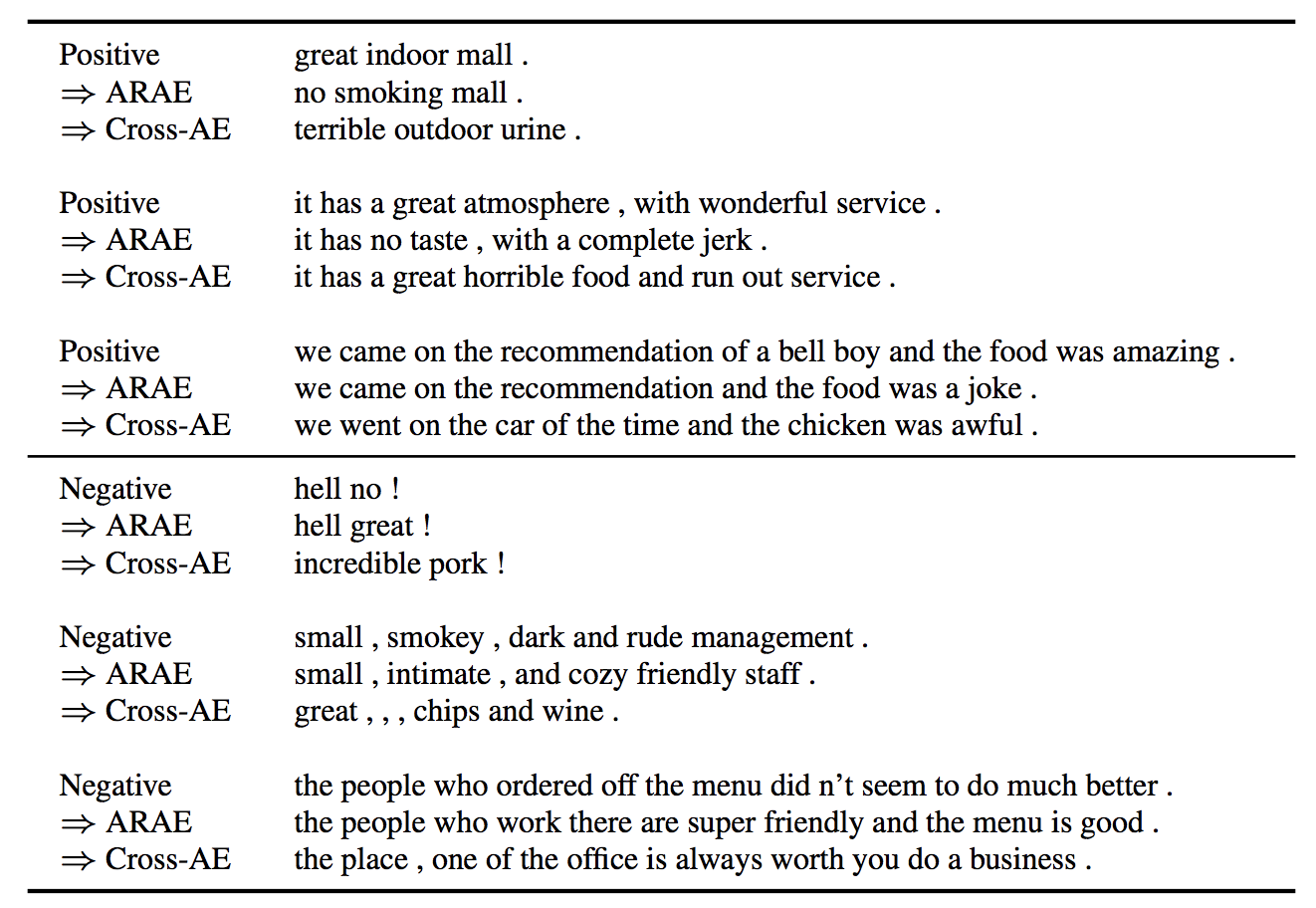
One task that has fascinated researchers is sentiment transfer: how can we control generation of the underlying meaning of a sentence (e.g. change its sentiment, topic etc.) through use and manipulation of a latent representation? I recently came across this paper titled Adversarially Regularized Autoencoders paper by Zhao et. al., where the authors attempt to apply Adversarial Autoencoders to discrete inputs, and perform sentiment and topic transfer. While the results are anywhere from questionable to comical to borderline workable, the algorithm itself is still an interesting, and insightful look into modern research in NLG, language modelling, and sentiment transfer.


Understanding the ARAE paper requires a bit of background knowledge about the methodologies that the ARAE was built up from. In 2014-15 led by the creation of GANs/VAEs, researchers first began to deep dive into direct-backpropagation generative models. For the past few years there’s been countless papers trying out different models of GAN/VAEs to improve them individually, while other papers attempted to find a unifying framework combining the best qualities of both, in a principled manner.
Progression of latent models to adversarial autoencoders
Adversarial Autoencoders
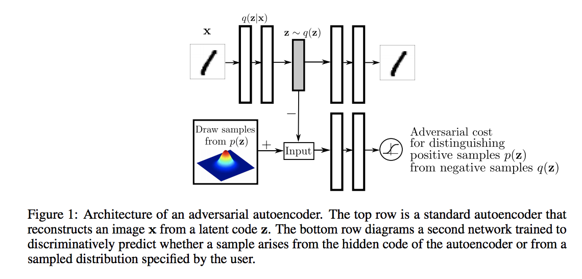
In 2015 Makhzani et. al. first proposed Adversarial Autoencoders (“AAE”). AAEs worked like VAEs: they take input data, encoded it, and attempted to learn a smooth latent distribution that could be decoded back to its original form. However, rather than smoothing the latent distribution through measuring (minimizing) KL, AAEs used adversarial training by creating an arbitrary prior (say Gaussian), and setting up a discriminator that would try to distinguish between the latent distribution created by the encoder, and that of the prior. Thus, through backprop the encoder would eventually shape its latent output to resemble the prior.

AAEs offered a few distinct advantages to VAEs and GANs. Not only did they seem to smooth the latent distribution a bit better than VAEs, they importantly did not require the exact functional form of the prior distribution in order to smooth the latent (since you just need to sample the prior in the adversarial training, rather than calculate the KL directly). The authors also demonstrated some interesting semi-supervised methods, unsupervised clustering, and dimensionality reduction techniques with AAEs.
Wasserstein GANs
In 2017 Arjovsky proposed Wasserstein GANs, which were GANs that used the Wasserstein metric to measure loss, which helped stabilize training and provided a more useful loss metric as related to generation quality. Here is a useful explanation, and I also wrote about WGANs in more detail in my last post.
Wasserstein Autoencoders
WAEs (Tolstikhin et. al. 2017) aimed to build up, and generalize the techniques used in WGANs and AAEs. There’s a lot going on here and it’s not quite essential to understand for ARAEs, but basically WAEs boil down to this:
Unlike a GAN a WAE has an encoder which gives you access to generating the latent space, which is useful. WAE generalizes AAEs because now you can use any cost function c and any divergence measure \(D_Z\), rather than say squared loss, or Wasserstein-1 distance, (such as in WGANs) due to…math I’m not going to get into (in short Kantorovich-Rubinstein duality holds only for Wasserstein-1, see the WGAN paper).
Adversarially Regularized Autoencoders
Alright, so if you’ve made it this far you’ve basically got everything you need to understand, with a couple of small twists to deal with discreteness. ARAEs are essentially AAEs, that use the WGAN (Wasserstein-1) adversarial setup to smooth its latent variables; it’s a variation of the generalized WAE, and different from the standard AAE which minimizes Wasserstein-2.
The main contribution is that the ARAE learns a prior through a parameterized generator. The authors chose to do this because the inflexible, arbitrary prior suffered from mode collapse. In vanilla AAEs you were just given that the prior \(P_Z\) was say, Gaussian. In the ARAE you take a simple random variable \(s \sim \mathcal{N}(0, 1)\), \(z = g_\theta(s)\) and you parameterize the latent distribution of Z through the generator neural net. Through adversarial training, the generator learns its own prior structure. Notice how AAEs in general move the adversarial training away from the input (pixel) space, to the latent space, which avoids the issue of discrete inputs for vanilla GANs.
References:
- [1] https://www.nytimes.com/interactive/2018/01/02/technology/ai-generated-photos.html
- [2] https://www.quora.com/What-is-the-REINFORCE-algorithm
- [3] https://www.reddit.com/r/MachineLearning/comments/40ldq6/generative_adversarial_networks_for_text/
